Exploiting Scaling Constants to Facilitate the Convergence of Indirect Trajectory Optimization Methods

Authors: Minduli C. Wijayatunga, Laura Pirovano, Roberto Armellin

Venue: Journal of Guidance, Control, and Dynamics (Engineering Note), Vol. 46, No. 5, May 2023

DOI: 10.2514/1.G007091

Indirect optimal control • Low-thrust • Continuation • EO→FO / EO→TO transitions • J2 + eclipses

Overview

Indirect (Pontryagin-based) methods can be extremely efficient and accurate for low-thrust trajectory optimisation, but in practice they are often bottlenecked by convergence sensitivity to the initial costate guess and discontinuities in bang–bang structures.

This note proposes a practical continuation strategy that uses scaling constants to transition from an energy-optimal (EO) solution into fuel-optimal (FO) and time-optimal (TO) problems. The goal is to obtain a “good enough” path for the optimiser to converge quickly, even when perturbations and eclipses are present.

What you get

• A simple EO→FO mapping via \(\beta_f\)
• A simple EO→TO mapping via \(\beta_t\)
• Fewer iterations / lower residuals in shooting solves
• Demonstrations across heliocentric + geocentric cases

Method

1) Solve an Energy-Optimal (EO) problem as the “bridge”

The EO problem is typically smoother than FO/TO and is used to obtain a robust initial guess for costates. Conceptually:

\[ \min_{\mathbf{u}(\cdot)} J_E \;\;=\;\; \int_{t_0}^{t_1} \|\mathbf{u}(t)\|^2 \, dt \quad \text{s.t. dynamics and boundary conditions.} \]

The EO solution provides a stable starting point (state + costates + switching structure cues) to initialise harder problems.

2) EO → Fuel-Optimal (FO) using \(\beta_f\)

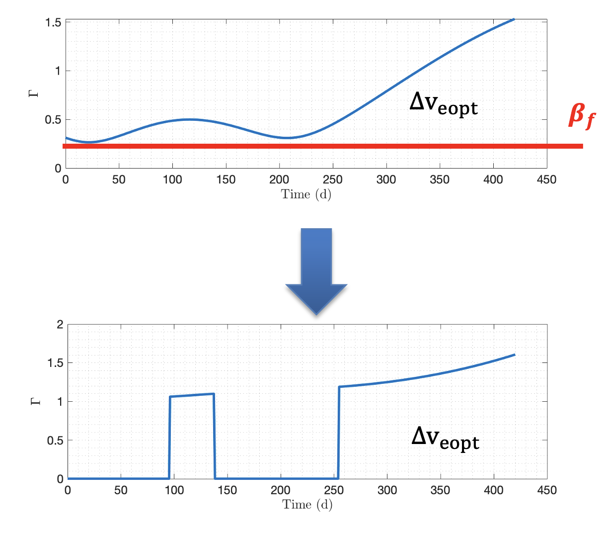
Fuel-optimal control tends toward bang–bang behaviour and can be difficult for indirect shooting methods without a good initialisation. Introduce a positive scaling constant \(\beta_f\) in the FO objective to promote a convenient thrust profile during the transition from EO:

\[ \min_{\mathbf{u}(\cdot)} J_F \;\;=\;\; \beta_f \int_{t_0}^{t_1} \|\mathbf{u}(t)\| \, dt \]

In this work, \(\beta_f\) is selected from the EO solution (via the EO-derived switching structure) so the continuation lands in a region where the FO shooting method converges with fewer iterations.

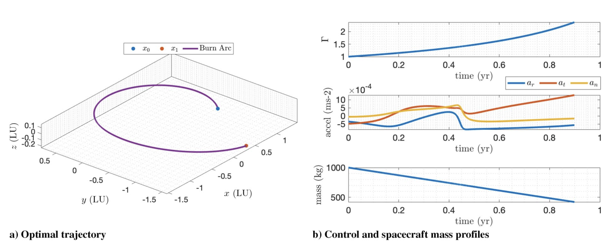
3) EO → Time-Optimal (TO) using \(\beta_t\)

For time-optimal problems, an EO solve with a free final time can provide a strong initial guess for flight time and costates. A constant scaling factor \(\beta_t\) is used to reduce residuals and improve convergence:

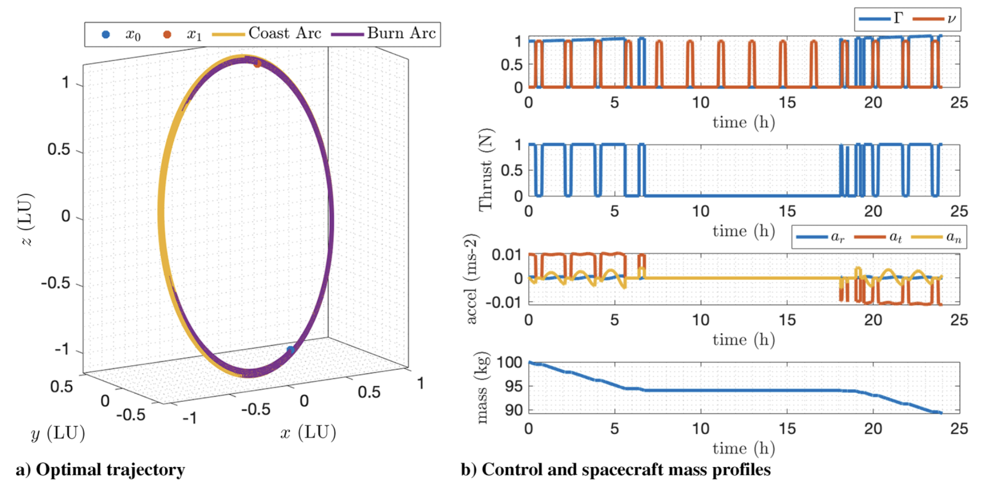
\[ \min_{\mathbf{u}(\cdot),\, t_1} J_T \;\;=\;\; \beta_t \int_{t_0}^{t_1} 1 \, dt \;=\; \beta_t (t_1 - t_0). \]

This EO-initialised continuation can be applied with Keplerian dynamics, and extended to perturbations (e.g., \(J_2\)) and eclipses.

EO-derived switching structure

A practical reason the energy-optimal (EO) problem is a useful “bridge” is that it reveals a proxy switching structure that closely resembles the on/off pattern that appears in fuel-optimal (FO) and time-optimal (TO) solutions. We use this EO-derived structure to initialise the indirect shooting solve and to choose the scaling constants \( \beta_f \) and \( \beta_t \) so the continuation lands in a region where the solver converges reliably.

Key idea

From the EO solution, construct a “switching indicator” using the EO control magnitude (or an equivalent EO switching function proxy). A simple representation is:

\[ s_E(t) \;=\; \|\mathbf{u}_E(t)\| \quad \Rightarrow \quad \text{burn at } t \text{ if } s_E(t) \ge s_{\mathrm{th}}. \]

This produces a time-partition (burn / coast arcs) that can be carried into FO/TO as an initial guess for the bang–bang pattern, including approximate arc boundaries.

In implementation, the EO-derived switching structure is used in two ways:

Initialise switching times / arc partitioning for the FO/TO shooting solve, reducing sensitivity to the initial costate guess.
Set continuation scaling so that the FO/TO costate magnitudes and the resulting switching function are well-conditioned during the transition (via \( \beta_f \) and \( \beta_t \)).

Determination of \(\beta_f\).

Implementation outline

EO to FO

Solve EO to obtain state/costate trajectories and switching cues.
Compute \(\beta_f\) from the EO solution, then solve FO using EO as the initial guess.

EO to TO

Solve EO with free final time to seed TOF, compute \(\beta_t\), then solve TO.
Optionally add \(J_2\) and eclipse modelling, keeping the continuation logic unchanged.

Results

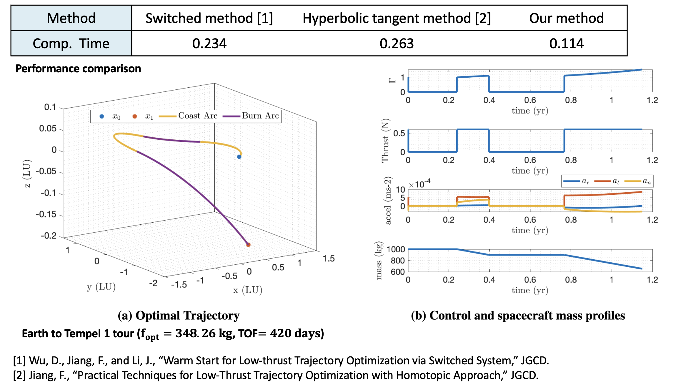
Headline takeaway: introducing \(\beta_f\) for FO and \(\beta_t\) for TO supports convergence and reduces practical tuning burden compared to “classical” indirect setups (e.g., default unity scaling).

Time- and fuel-optimal solutions (Table 9)

Values reproduced into a web-native table.

Mission	FO flight time (d)	FO fuel (kg)	FO compute (s)	\(\beta_f\)	TO flight time (d)	TO fuel (kg)	TO compute (s)	\(\beta_t\)
Earth → Tempel 1	420.00	348.26	0.114	0.4781	328.13	578.18	0.208	21.3486
Earth → Dionysus	3534.00	1280.70	0.425	0.5389	1848.89	1737.53	0.733	2.9195
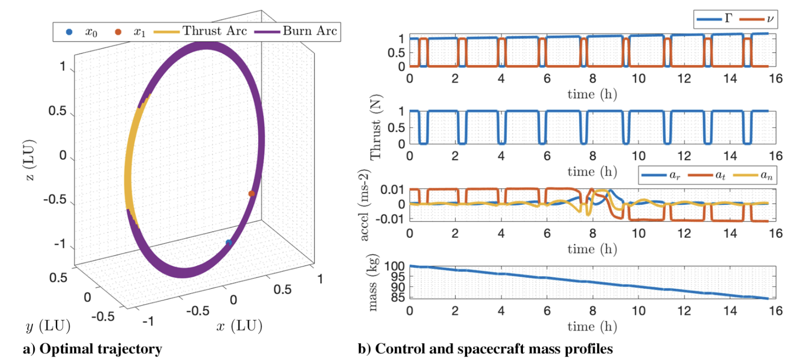
Space debris (geocentric)	1.00	11.09	75.600	0.4886	0.654	15.74	55.320	27.1080

• \(\beta_f\) supports EO→FO continuation and helps reduce iterations to convergence.
• \(\beta_t\) supports EO-initialised TO solves by reducing residuals / improving convergence behaviour.
• Demonstrations include heliocentric transfers and a geocentric debris-to-debris case (with perturbations/eclipses variants discussed).

Results

Cite this work

BibTeX

@article{Wijayatunga2023ScalingConstants,
  title   = {Exploiting Scaling Constants to Facilitate the Convergence of Indirect Trajectory Optimization Methods},
  author  = {Wijayatunga, Minduli C. and Armellin, Roberto and Pirovano, Laura},
  journal = {Journal of Guidance, Control, and Dynamics},
  volume  = {46},
  number  = {5},
  pages   = {958--969},
  year    = {2023},
  doi     = {10.2514/1.G007091}
}

If you prefer, swap the citation key or adjust page ranges to match your preferred bibliography format.